(本ページはTensorFlowを理解していない、pythonも使ったことない、OpenCVも先日使い始めたばかりな者が書いていますので誤りを含むかもしれません)
tensorflowとOpenCVはdocker上にセットアップした方が楽そうです。 以下も参照ください。 https://qiita.com/summer4an/items/5a10fe8cc13476f09963
サーバ上で試しに判別してみていただける環境を用意しました。 よければアクセスしてみてください。 https://www.nakajimadevnakajima.info/va/kyohin/form.html
コードを以下に置きました。 https://www.nakajimadevnakajima.info/va/kyonyuu_hinnyuu_hanbetu.zip
ディープラーニングや画像処理の勉強をしたい+そういえば巨乳顔というものがあるらしい →ディープラーニングで顔写真から巨乳かどうかを判別してみよう!
一応まじめに考えて、顔がふっくらしていれば胸も大きい可能性が高いだろうから、顔のつくりと胸の大きさには相関があるだろう。 顔の丸さやまぶたの肉の付き方等の顔の特徴を数値化してディープラーニングさせれば良さそう。 ということでやってみた。
巨乳な方はこの辺りから。
貧乳な方はこの辺りから。
ただし外国の方は顔のつくりが異なりすぎて学習がうまくいく気がしないので日本の方に限定。 また、AV女優の方は整形や豊胸の可能性が高そうなので除いた(と思う)。
巨乳の方は全250名程度、貧乳の方は全160名程度。リストは自粛。欲しければご連絡ください。
適当な画像検索サイトからスクレイピング。今回はbing画像検索を使った。
#!/bin/bash

#画像ゲッター

#引数で人名を与えると、temp_ほげほげ_gazou/gazou_00001.jpg等という連番で画像を保存してくれる。
#  getter "ほげほげ"
function getter() {
  for name in "$@"; do
    echo -e '\n\n\n\n'

    targettext_encoded=`echo "$name" | perl -MURI::Escape -lne 'print uri_escape($_)'`
    url='https://www.bing.com/images/search?FORM=HDRSC2&q='${targettext_encoded}
    echo target is "${name}" "${url}"

    if [ -d temp_${name}_gazou ]; then
      echo already downloaded temp_${name}_gazou
      continue
    fi

    mkdir temp_${name}_gazou
    pushd temp_${name}_gazou

    wget -r -l 1 -H "${url}"
    rm -rf tse1.mm.bing.net/ tse2.mm.bing.net/ tse3.mm.bing.net/ tse4.mm.bing.net/ www.bing.com/ www.bingfudosan.jp/
    find ./ -not -name '*.jpg' -a -not -name '*.jpeg' -a -not -name '*.JPG' -type f -print0 | xargs -0 rm

    find ./ -type f | awk '{printf("mv '"'"'%s'"'"' gazou_%05d.jpg\n", $0, NR);}' > ../temp_${name}_gazou_filename_henkan.sh
    bash ../temp_${name}_gazou_filename_henkan.sh
    find ./ -maxdepth 1 -type d -print0 | xargs -0 rm -rf

    popd

    #連続でwgetするのを防ぐため。
    sleep 5
  done
}

getter "ほげほげ子" "もげもげ美" ・・・
以下で実行。
$ ./jpggetter.sh
巨乳の方は全250名5600枚程度、貧乳の方は全160名3500枚程度集まった。
この辺を参考に。
ただし複数人の顔が検出された場合はそれぞれの名前が分からないので捨てるようにしている。
都合により、1ファイルに対する顔の切り抜きはwindows上のOpenCVを使ったexeで、それを各顔画像ファイルに対して実行するのはcygwin上でシェルスクリプトで行った。 windows上でOpenCVするためのメモはここ。
//実行方法は以下。
//  hoge.exe ターゲットのファイル名 出力ファイル名 cascadeファイル名
//戻り値は、0が正常終了、100より下は引数不足等の実行時の異常、100以上はOpenCVは走ったが検出出来なかった等

#include "stdafx.h"
#include <opencv2/opencv.hpp>
#include <iostream>
#include <windows.h>

using namespace std;
using namespace cv;

#define FACE_KAKUDAI_WARIAI 1.2 //例えば検出された顔が100px四方だとしたら、100×FACE_KAKUDAI_WARIAIpxのサイズで切り抜く

int main(int argc, char const *argv[]) {
	if(argc!=4){
		printf("error. too few argument.\n");
		exit(1);
	}
	printf("target file is %s\n", argv[1]);

	Mat image = imread(argv[1]);
	if(image.data==NULL){
		printf("error. can not read source picture file.\n");
		exit(2);
	}
	printf("image size width=%d height=%d\n", image.size().width, image.size().height);

	string cascade_filename = argv[3];
	CascadeClassifier cascade;
	if(cascade.load(cascade_filename)!=true){
		printf("error. can not read cascade file.\n");
		exit(3);
	}

	vector<Rect> faces;
	cascade.detectMultiScale(image, faces, 1.1, 3, 0);
	printf("detect %zu faces.\n", faces.size());

	if(faces.size()!=1){
		printf("too many faces or no faces detected. exit.\n");
		exit(100);
	}

	for (int i = 0; i < faces.size(); i++) {
		printf("face[%d] x=%d y=%d width=%d height=%d\n", i, faces[i].x, faces[i].y, faces[i].width, faces[i].height);

		//切り抜くサイズを少し大きくした時に画像をはみ出るかどうか確認。
		int kakudai_size = (int)(faces[i].width * (FACE_KAKUDAI_WARIAI-1) / 2); //左右で拡大するので2で割っている。
		int kirinuki_x = faces[i].x-kakudai_size;
		int kirinuki_y = faces[i].y-kakudai_size;
		int kirinuki_width  = faces[i].width + kakudai_size*2;
		int kirinuki_height = faces[i].height+ kakudai_size*2;
		if( kirinuki_x<0 ||
			kirinuki_y<0 ||
			image.size().width  <= kirinuki_x+kirinuki_width ||
			image.size().height <= kirinuki_y+kirinuki_height ){
			printf("face[%d] located on corner. skip.\n", i);
			exit(101);
		}

		Mat cut_img(image, Rect(kirinuki_x, kirinuki_y, kirinuki_width, kirinuki_height));
		imwrite(argv[2], cut_img);
		printf("face[%d] outputed as \"%s\"\n", i, argv[2]);

		rectangle(image, Point(faces[i].x, faces[i].y), Point(faces[i].x + faces[i].width, faces[i].y + faces[i].height), Scalar(0, 200, 0), 1, CV_AA);
		rectangle(image, Point(kirinuki_x, kirinuki_y), Point(kirinuki_x + kirinuki_width, kirinuki_y + kirinuki_height), Scalar(200, 0, 0), 1, CV_AA);
	}

	//imshow("detect face", image);
	//waitKey(0);

	return 0;
}
#!/bin/bash

#顔部分だけ切り抜く。
#「./faces/temp_*_gazou/」以下の各gazou_*.jpgに対して処理を実行。
#「./faces/temp_*_gazou/face_gazou_00001.jpg」等のファイルができる。

CASCADE_FILENAME='(haarcascade_frontalface_alt2.xmlへのパス)'

for i in ./faces/temp_*_gazou; do
  echo -e '\n\n\n\n'
  echo target dir $i
  pushd $i

  for j in gazou_*.jpg; do
    echo -e '\n'
    echo -e 'target dir is' "$i" ' target file is' "$j"

    if [ -f face_$j ]; then
      echo 'already detected face. skip'
      continue
    fi

    echo target file $j

    ./face_kirinuki.exe $j face_$j ${CASCADE_FILENAME}

    #もし判別に失敗してface_*.jpgのファイルができなかった場合、空のファイルを作る。
    if [ $? -ne 0 ]; then
      touch face_$j
      continue
    fi

    #サイズを同じにする
    mogrify -geometry 256x256 face_$j
  done

  popd
done
以下で実行。
$ ./face_kirinuki.sh
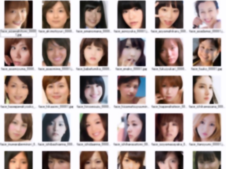
終わったら目で見て誤検知しているもの、顔の一部しか写っていないもの、正面向きでないもの、そもそも全然違う人の写真は除去しておく。
巨乳の方は全250名2500枚程度、貧乳の方は全160名1700枚程度になった。
ローカルで動く顔の丸さ等の特徴抽出用ライブラリがないか探してみたが見つけられず。自前で特徴量を抽出するのは諦め。 webサービスならこの辺りがある模様。
特徴量を求めてからディープラーニングのフレームワークのChainerやTensorFlowに食わせようと考えていたが、そもそも何も考えずにぶっこむだけで画像分類してくれるっぽいのでやってみる。
Chainerはなぜかうまく動かなかったのでTensorFlowで。
以下公式サイトの「Pip Installation」を参照。pythonのライブラリはpipというものを使って入れるらしい。
$ sudo apt-get install python-pip python-dev
$ sudo pip install --upgrade https://storage.googleapis.com/tensorflow/linux/cpu/tensorflow-0.6.0-cp27-none-linux_x86_64.whl
virtual box上Ubuntu14.04 64bitを使用。 ろくなGPUが載っていないのでCPU版をセットアップした。特に難しくない。 「Run TensorFlow from the Command Line」の箇所を参照し動作確認しておく。
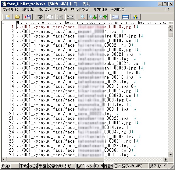
集めた顔写真ファイル群から、学習用の方と、テスト用の方と、最後に巨乳か判別するお試し用の方を分けておく。 学習用はface_filelist_train.txt、テスト用はface_filelist_test.txtに、以下のような形式でリストアップ。
  (ファイルパス) (分類 巨乳なら1、貧乳なら0)
  ./faces/face_hogeko_00001.jpg 1
  ./faces/face_mogemi_00001.jpg 0
  ・・・
もしかしたらリストはシャッフルしておいた方が良いかも。前半が巨乳、後半が貧乳等並んでいると学習が進まないかも(試行錯誤していた時だったので他の原因かもしれない)。sortの-Rオプションを使えばOK。
以下によると学習用には60~80%割り当てると良いとのこと。
学習用に3000枚、テスト用に1200枚を割り当てた。
コードは以下の「コード全体」から拝借。
ただ稀に「ReluGrad input is not finite. : Tensor had NaN values」というエラーで異常終了することがあったので、以下参考に異常処理を追加。
#!/usr/bin/env python
# -*- coding: utf-8 -*-

import sys
import cv2
import numpy as np
import tensorflow as tf
import tensorflow.python.platform

NUM_CLASSES = 2
IMAGE_SIZE = 28
IMAGE_PIXELS = IMAGE_SIZE*IMAGE_SIZE*3

flags = tf.app.flags
FLAGS = flags.FLAGS
flags.DEFINE_string('train', 'face_filelist_train.txt', 'File name of train data')
flags.DEFINE_string('test', 'face_filelist_test.txt', 'File name of train data')
flags.DEFINE_string('train_dir', './logdata', 'Directory to put the training data.')
flags.DEFINE_integer('max_steps', 100, 'Number of steps to run trainer.')
flags.DEFINE_integer('batch_size', 10, 'Batch size'
                     'Must divide evenly into the dataset sizes.')
flags.DEFINE_float('learning_rate', 1e-4, 'Initial learning rate.')

def inference(images_placeholder, keep_prob):
    """ 予測モデルを作成する関数

    引数:
      images_placeholder: 画像のplaceholder
      keep_prob: dropout率のplace_holder

    返り値:
      y_conv: 各クラスの確率(のようなもの)
    """
    # 重みを標準偏差0.1の正規分布で初期化
    def weight_variable(shape):
      initial = tf.truncated_normal(shape, stddev=0.1)
      return tf.Variable(initial)

    # バイアスを標準偏差0.1の正規分布で初期化
    def bias_variable(shape):
      initial = tf.constant(0.1, shape=shape)
      return tf.Variable(initial)

    # 畳み込み層の作成
    def conv2d(x, W):
      return tf.nn.conv2d(x, W, strides=[1, 1, 1, 1], padding='SAME')

    # プーリング層の作成
    def max_pool_2x2(x):
      return tf.nn.max_pool(x, ksize=[1, 2, 2, 1],
                            strides=[1, 2, 2, 1], padding='SAME')

    # 入力を28x28x3に変形
    x_image = tf.reshape(images_placeholder, [-1, 28, 28, 3])

    # 畳み込み層1の作成
    with tf.name_scope('conv1') as scope:
        W_conv1 = weight_variable([5, 5, 3, 32])
        b_conv1 = bias_variable([32])
        h_conv1 = tf.nn.relu(conv2d(x_image, W_conv1) + b_conv1)

    # プーリング層1の作成
    with tf.name_scope('pool1') as scope:
        h_pool1 = max_pool_2x2(h_conv1)

    # 畳み込み層2の作成
    with tf.name_scope('conv2') as scope:
        W_conv2 = weight_variable([5, 5, 32, 64])
        b_conv2 = bias_variable([64])
        h_conv2 = tf.nn.relu(conv2d(h_pool1, W_conv2) + b_conv2)

    # プーリング層2の作成
    with tf.name_scope('pool2') as scope:
        h_pool2 = max_pool_2x2(h_conv2)

    # 全結合層1の作成
    with tf.name_scope('fc1') as scope:
        W_fc1 = weight_variable([7*7*64, 1024])
        b_fc1 = bias_variable([1024])
        h_pool2_flat = tf.reshape(h_pool2, [-1, 7*7*64])
        h_fc1 = tf.nn.relu(tf.matmul(h_pool2_flat, W_fc1) + b_fc1)
        # dropoutの設定
        h_fc1_drop = tf.nn.dropout(h_fc1, keep_prob)

    # 全結合層2の作成
    with tf.name_scope('fc2') as scope:
        W_fc2 = weight_variable([1024, NUM_CLASSES])
        b_fc2 = bias_variable([NUM_CLASSES])

    # ソフトマックス関数による正規化
    with tf.name_scope('softmax') as scope:
        y_conv=tf.nn.softmax(tf.matmul(h_fc1_drop, W_fc2) + b_fc2)

    # 各ラベルの確率のようなものを返す
    return y_conv

def loss(logits, labels):
    """ lossを計算する関数

    引数:
      logits: ロジットのtensor, float - [batch_size, NUM_CLASSES]
      labels: ラベルのtensor, int32 - [batch_size, NUM_CLASSES]

    返り値:
      cross_entropy: 交差エントロピーのtensor, float

    """

    # 交差エントロピーの計算
    #cross_entropy = -tf.reduce_sum(labels*tf.log(logits)) 異常処理 http://qiita.com/ikki8412/items/3846697668fc37e3b7e0
    cross_entropy = -tf.reduce_sum(labels*tf.log(tf.clip_by_value(logits,1e-10,1.0)))
    # TensorBoardで表示するよう指定
    tf.scalar_summary("cross_entropy", cross_entropy)
    return cross_entropy

def training(loss, learning_rate):
    """ 訓練のOpを定義する関数

    引数:
      loss: 損失のtensor, loss()の結果
      learning_rate: 学習係数

    返り値:
      train_step: 訓練のOp

    """

    train_step = tf.train.AdamOptimizer(learning_rate).minimize(loss)
    return train_step

def accuracy(logits, labels):
    """ 正解率(accuracy)を計算する関数

    引数:
      logits: inference()の結果
      labels: ラベルのtensor, int32 - [batch_size, NUM_CLASSES]

    返り値:
      accuracy: 正解率(float)

    """
    correct_prediction = tf.equal(tf.argmax(logits, 1), tf.argmax(labels, 1))
    accuracy = tf.reduce_mean(tf.cast(correct_prediction, "float"))
    tf.scalar_summary("accuracy", accuracy)
    return accuracy

if __name__ == '__main__':
    # ファイルを開く
    f = open(FLAGS.train, 'r')
    # データを入れる配列
    train_image = []
    train_label = []
    for line in f:
        # 改行を除いてスペース区切りにする
        line = line.rstrip()
        l = line.split()
        # データを読み込んで28x28に縮小

        print "aaaaa line[%s] %s %s"%(line,l[0],l[1])

        img = cv2.imread(l[0])
        img = cv2.resize(img, (28, 28))
        # 一列にした後、0-1のfloat値にする
        train_image.append(img.flatten().astype(np.float32)/255.0)
        # ラベルを1-of-k方式で用意する
        tmp = np.zeros(NUM_CLASSES)
        tmp[int(l[1])] = 1
        train_label.append(tmp)
    # numpy形式に変換
    train_image = np.asarray(train_image)
    train_label = np.asarray(train_label)
    f.close()

    f = open(FLAGS.test, 'r')
    test_image = []
    test_label = []
    for line in f:
        line = line.rstrip()
        l = line.split()
        img = cv2.imread(l[0])
        img = cv2.resize(img, (28, 28))

        print "aaaaa2 line[%s] %s %s"%(line,l[0],l[1])

        test_image.append(img.flatten().astype(np.float32)/255.0)
        tmp = np.zeros(NUM_CLASSES)
        tmp[int(l[1])] = 1
        test_label.append(tmp)
    test_image = np.asarray(test_image)
    test_label = np.asarray(test_label)
    f.close()

    with tf.Graph().as_default():
        # 画像を入れる仮のTensor
        images_placeholder = tf.placeholder("float", shape=(None, IMAGE_PIXELS))
        # ラベルを入れる仮のTensor
        labels_placeholder = tf.placeholder("float", shape=(None, NUM_CLASSES))
        # dropout率を入れる仮のTensor
        keep_prob = tf.placeholder("float")

        # inference()を呼び出してモデルを作る
        logits = inference(images_placeholder, keep_prob)
        # loss()を呼び出して損失を計算
        loss_value = loss(logits, labels_placeholder)
        # training()を呼び出して訓練
        train_op = training(loss_value, FLAGS.learning_rate)
        # 精度の計算
        acc = accuracy(logits, labels_placeholder)

        # 保存の準備
        saver = tf.train.Saver()
        # Sessionの作成
        sess = tf.Session()
        # 変数の初期化
        sess.run(tf.initialize_all_variables())
        # TensorBoardで表示する値の設定
        summary_op = tf.merge_all_summaries()
        summary_writer = tf.train.SummaryWriter(FLAGS.train_dir, sess.graph_def)

        # 訓練の実行
        for step in range(FLAGS.max_steps):
            for i in range(len(train_image)/FLAGS.batch_size):
                # batch_size分の画像に対して訓練の実行
                batch = FLAGS.batch_size*i
                # feed_dictでplaceholderに入れるデータを指定する
                sess.run(train_op, feed_dict={
                  images_placeholder: train_image[batch:batch+FLAGS.batch_size],
                  labels_placeholder: train_label[batch:batch+FLAGS.batch_size],
                  keep_prob: 0.5})

            # 1 step終わるたびに精度を計算する
            train_accuracy = sess.run(acc, feed_dict={
                images_placeholder: train_image,
                labels_placeholder: train_label,
                keep_prob: 1.0})
            print "step %d, training accuracy %g"%(step, train_accuracy)

            # 1 step終わるたびにTensorBoardに表示する値を追加する
            summary_str = sess.run(summary_op, feed_dict={
                images_placeholder: train_image,
                labels_placeholder: train_label,
                keep_prob: 1.0})
            summary_writer.add_summary(summary_str, step)

    # 訓練が終了したらテストデータに対する精度を表示
    print "test accuracy %g"%sess.run(acc, feed_dict={
        images_placeholder: test_image,
        labels_placeholder: test_label,
        keep_prob: 1.0})

    # 最終的なモデルを保存
    save_path = saver.save(sess, "model.ckpt")
以下で実行。
$ python gakusyuu.py
Core i7 2.1GHz win7のノートPC上で、virtual boxでubuntu14.04に4CPU 4GBメモリ割り当てて動かした上で実行。100回の学習で30分程度で終わる。
学習の途中経過は以下実行した後、ブラウザで「 http://localhost:6006 」にアクセスすれば見れる。
  $ tensorboard --logdir=(ログファイルのあるディレクトリの絶対パス)
  $ tensorboard --logdir=/home/hoge/kyonyuu_hanbetu/logdata
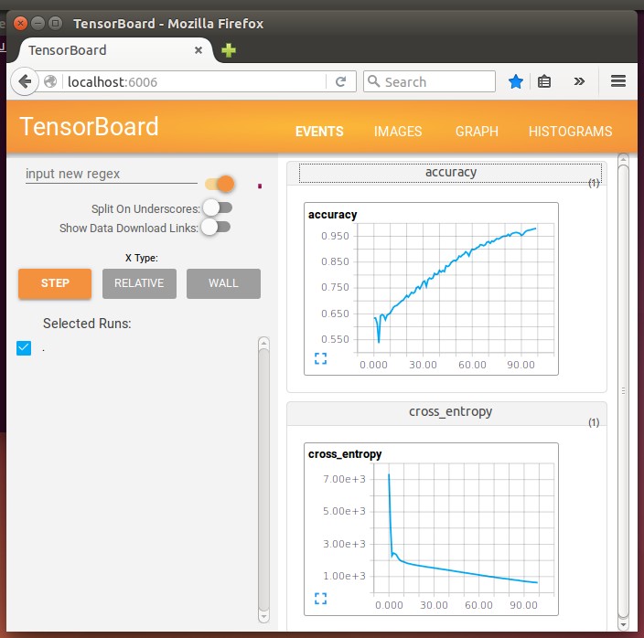
最終的に学習用の顔に対しては「step 99, training accuracy 0.980135」になった。
ただテスト用の顔に対しての判定結果が「test accuracy 0.534127」とのこと。ほぼ判別できていない…
とりあえず学習用にもテスト用にも使っていない方の顔写真で判定してみる。 コードは以下の「画像に対して予想ラベルを表示する」の下から拝借。
メインはpythonコードで、シェルスクリプトではログを記録しているだけ。
#!/usr/bin/env python
#! -*- coding: utf-8 -*-

import sys
import numpy as np
import tensorflow as tf
import cv2


NUM_CLASSES = 2
IMAGE_SIZE = 28
IMAGE_PIXELS = IMAGE_SIZE*IMAGE_SIZE*3

def inference(images_placeholder, keep_prob):
    """ モデルを作成する関数

    引数:
      images_placeholder: inputs()で作成した画像のplaceholder
      keep_prob: dropout率のplace_holder

    返り値:
      cross_entropy: モデルの計算結果
    """
    def weight_variable(shape):
      initial = tf.truncated_normal(shape, stddev=0.1)
      return tf.Variable(initial)

    def bias_variable(shape):
      initial = tf.constant(0.1, shape=shape)
      return tf.Variable(initial)

    def conv2d(x, W):
      return tf.nn.conv2d(x, W, strides=[1, 1, 1, 1], padding='SAME')

    def max_pool_2x2(x):
      return tf.nn.max_pool(x, ksize=[1, 2, 2, 1],
                            strides=[1, 2, 2, 1], padding='SAME')

    x_image = tf.reshape(images_placeholder, [-1, 28, 28, 3])

    with tf.name_scope('conv1') as scope:
        W_conv1 = weight_variable([5, 5, 3, 32])
        b_conv1 = bias_variable([32])
        h_conv1 = tf.nn.relu(conv2d(x_image, W_conv1) + b_conv1)

    with tf.name_scope('pool1') as scope:
        h_pool1 = max_pool_2x2(h_conv1)

    with tf.name_scope('conv2') as scope:
        W_conv2 = weight_variable([5, 5, 32, 64])
        b_conv2 = bias_variable([64])
        h_conv2 = tf.nn.relu(conv2d(h_pool1, W_conv2) + b_conv2)

    with tf.name_scope('pool2') as scope:
        h_pool2 = max_pool_2x2(h_conv2)

    with tf.name_scope('fc1') as scope:
        W_fc1 = weight_variable([7*7*64, 1024])
        b_fc1 = bias_variable([1024])
        h_pool2_flat = tf.reshape(h_pool2, [-1, 7*7*64])
        h_fc1 = tf.nn.relu(tf.matmul(h_pool2_flat, W_fc1) + b_fc1)
        h_fc1_drop = tf.nn.dropout(h_fc1, keep_prob)

    with tf.name_scope('fc2') as scope:
        W_fc2 = weight_variable([1024, NUM_CLASSES])
        b_fc2 = bias_variable([NUM_CLASSES])

    with tf.name_scope('softmax') as scope:
        y_conv=tf.nn.softmax(tf.matmul(h_fc1_drop, W_fc2) + b_fc2)

    return y_conv

if __name__ == '__main__':
    test_image = []
    filenames = []
    for i in range(1, len(sys.argv)):
        img = cv2.imread(sys.argv[i])
        img = cv2.resize(img, (28, 28))
        test_image.append(img.flatten().astype(np.float32)/255.0)
        filenames.append(sys.argv[i])
    test_image = np.asarray(test_image)

    images_placeholder = tf.placeholder("float", shape=(None, IMAGE_PIXELS))
    labels_placeholder = tf.placeholder("float", shape=(None, NUM_CLASSES))
    keep_prob = tf.placeholder("float")

    logits = inference(images_placeholder, keep_prob)
    sess = tf.InteractiveSession()

    saver = tf.train.Saver()
    sess.run(tf.initialize_all_variables())
    saver.restore(sess, "model.ckpt")

    for i in range(len(test_image)):
        pred = np.argmax(logits.eval(feed_dict={
            images_placeholder: [test_image[i]],
            keep_prob: 1.0 })[0])
        pred2 = logits.eval(feed_dict={
            images_placeholder: [test_image[i]],
            keep_prob: 1.0 })[0]
        print filenames[i],pred,"{0:10.8f}".format(pred2[0]),"{0:10.8f}".format(pred2[1])
#!/bin/bash
python ./hanbetu__all_file.py "$@" >> log_hanbetu_`date +%Y%m%d_%H%M%S`.txt
以下で実行。
$ ./hanbetu_all.sh (判別したいファイル 複数)
log_hanbetu_XXX.txtに結果が書き込まれ、巨乳と判別したものには1が、貧乳と判別したものには0がつく。また、巨乳の可能性と貧乳の可能性も数値で表示される。
巨乳の方全8名84枚、貧乳の方全8名81枚に対して実行。 結果は以下。
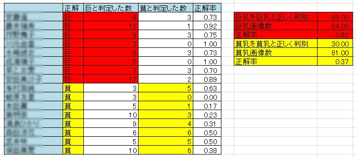
巨乳の方だけ見るとよさ気だが、単に多くを巨乳と判別しているだけか…? ただ巨乳の方で高い確率で当てている方もいるので、当てやすい顔の方なのかも。
いまいちうまくいったか微妙。 敗因として思いつくのは以下。
もしうまく判別出来ていたらこんな応用ができるかも?
気づいたこと。